Dividing a hydronic system in modules

The terminals in the figure 1 form a module. A disturbance external to the module causes a variation in the differential pressure across A and B. Since the flow depends on the differential pressure, the flows in all terminals change in the same proportion.

​​​

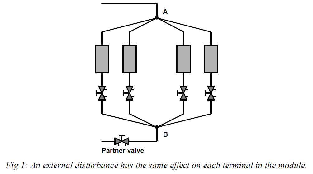
The flow through these terminals can therefore be monitored through measurement of the flow in just one of them, which can serve as a reference. A balancing valve common to all terminals can compensate for the effect of the external disturbance on the terminal flows in the module. We call this common valve the Partner Valve.

However, terminals are normally connected as in figure 2. The water flow through each terminal depends on the differential pressure between A and L. Any modification of this pressure affects the flow in each terminal in the same proportion.

​​

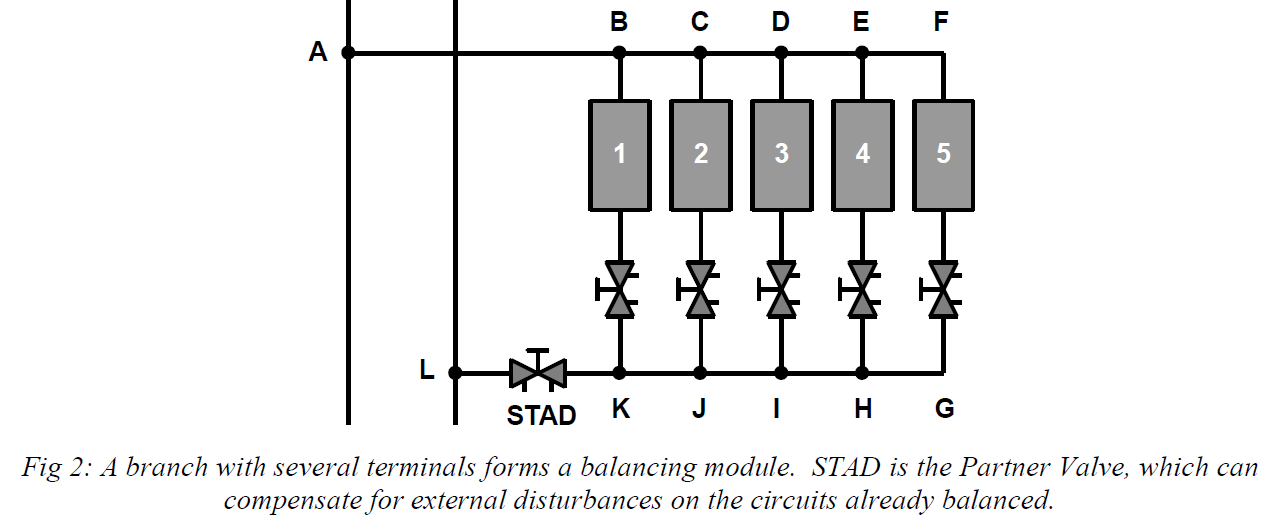
But what happens if we create a disturbance that is internal to the module, for instance by closing the balancing valve of terminal 3?

This will strongly influence the flows in pipes lines CD and IJ, and thus the pressure loss in these pipe lines. The differential pressure between E and H will change noticeably, which will affect the flows in terminals 4 and 5 in the same proportion.

The fact that terminal 3 is closed has little effect on the total flow in the pipe lines AB and KL. The pressure losses in these pipe lines change very little. The differential pressure between B and K is changed only somewhat and terminal 1 will not react to the disturbance in the same proportion as terminals 4 and 5. Thus, the law of proportional flow change does not apply for internal disturbances (as shown in figure 3).

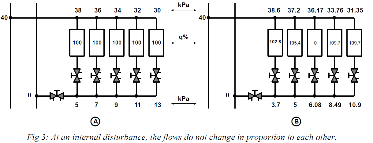
However, the water flows change in proportion in a module only if all the pressure drops depend on the flow q according to the same relation everywhere in the module. This is not true in reality because for the pipes the pressure drop depends on q^1.87.while it depends on q² in valves. For low flows, the circulation can become laminar and the pressure drop becomes linearly proportional to the flow. The law of proportionality can be used only to detect deviations around design values. This is one of the reasons why the most accurate balancing method is the Compensated Method as the design flows are maintained during the balancing process of each module.

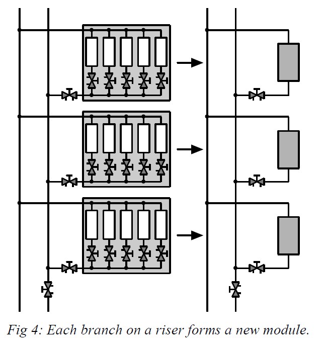
When the terminals on a branch are balanced against themselves, you may see the branch as a "black box", i.e. a module. Its components react proportionally to flow adjustment external to the module. The Partner Valve can easily compensate such disturbances.
In the next step, the branch modules are balanced against each other with the riser balancing valve as the Partner Valve. After this, all modules on the riser form a larger module, whose flow can be adjusted with the riser’s balancing valve. Finally, the risers are balanced against each other with each riser as a module and the balancing valve on the main pipe line as the Partner Valve.

Figure 5 shows two modules. The numbers indicate the design pressure loss in each terminal and the pressure loss in each balancing valve. Both modules are balanced. In both cases the differential pressure on each terminal is the required one to obtain design flow. The pressure losses are differently distributed between the balancing valves of the terminals and the Partner Valve.

Which balancing is the better of the two?

Optimum balancing means two things: (1) that the authority of the control valves is maximised for exact control, and that (2) pump oversizing is revealed so that pump head and thereby pumping costs can be minimised. Optimum balancing is obtained when the smallest possible pressure loss is taken in the balancing valves of the terminals (at least 3 kPa to allow precise flow measurement). Any remaining excess pressure is taken in the Partner Valve.

Balancing to obtain pressure losses as in (b) in the figure is thus the best, since the pressure loss is then the lowest admissible in all balancing valves on the terminals to obtain the design flows. Note that optimum balancing is only possible when the required Partner Valves are installed.

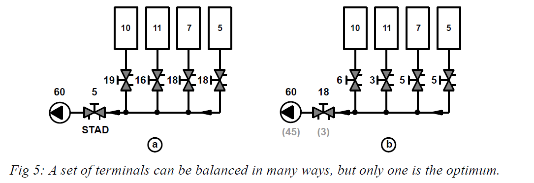
The Partner Valve reveals the excess of differential pressure. The pump speed for instance can be decreased correspondingly and the partner valve reopened. In example “b”, the pressure drop in the Partner Valve and the pump head can be reduced both by 15 kPa, decreasing the pumping costs by 25%.

The conclusion is that balancing valves should be installed to split the system in modules that can be balanced independently of the rest of the plant. Thus, each terminal, each​​ branch, each riser, each main and each production unit should be equipped with a balancing valve.

It is then simple to compensate for changes relative to the drawings, for any construction errors, and for oversizing. This saves time and allows optimum balancing. Furthermore, the plant can be balanced and commissioned in stages, without having to rebalance when the plant is completed.

The balancing valves are also used for troubleshooting and shut-off during service and maintenance.

We have considered the advantages of hydronic balancing. Before studying balancing procedures, the precision with which flows have to be adjusted has to be defined.

In practice, the flow adjustment precision to be achieved depends on the precision to be obtained on the room temperatur​e. This precision depends also on other factors such as the control of the supply water temperature and the ratio between the required and installed coil capacity. Some specifications stipulate a required water flow accuracy of between +0 and +5%. There is no technical justification for this severity. This requirement is even more surprising that little care appears to be taken about the actual temperature of the supply water to remote units. Particularly, in the case of variable flow distributions, the supply water temperature is certainly not the same at the beginning and at the end of the circuit, and the influence of this water temperature is not negligible. Furthermore, water flows are frequently calculated based on required capacity and they are rarely corrected as a function of the really installed capacity. Oversizing of the terminal unit by 25% should normally be compensated by a water flow reduction in the order of 40%. If this is not done, there is no point in adjusting the water flow to within 5% of accuracy while the required water flow is defined with an initial error of 40%.

An underflow cannot be compensated by the control loop, and has a direct effect on the environment under maximum load conditions; it must therefore be limited. An overflow has no direct consequence on the environment since in theory, the control loop can compensate for it. We may be tempted to accept overflows, especially when they have little effect on the room temperature. This would neglect the pernicious effect of overflows. When the control valves are fully open, for example when starting up the plant, the overflows produce underflows elsewhere and it is impossible to obtain the required water temperature at high loads, due to incompatibility between production and distribution flows. Overflows must therefore also be limited. This is why it is logical to penalise underflows and overflows with the same factor and to adopt a general precision rule in the form ±x%.

Fortunately, when the flow is situated close to the design value, it has no dramatic effect on the room temperature. By accepting a deviation of ± 0.5°C on the room temperature at full load due to water flow inaccuracy, the value of x, with a certain safety fact​ is in the order of:​

t_sc : Design supply water temperature.

t_ic : Design room temperature.

t_rc : Design return water temperature.

t_ec : Design outdoor temperature.

a_ic : Effect of internal heat on the room temperature.

Examples:

Heating- t_sc = 80°C; t_rc = 60°C; t_ic = 20°C; t_ec = -10°C; a_ic = 2°C; x = ±10%.

Cooling- t_sc = 6°C; t_rc = 12°C; t_ic = 22°C; tec = 35°C; aic = 5°C; x = ±15%.